Pivot tables are one of Excel’s most powerful features. They allow you to quickly summarize large amounts of data, making it easy to analyze trends, compare categories, and extract meaningful insights from your data.
In this tutorial, we’ll guide you through the steps to create a pivot table in Excel, along with examples to demonstrate different use cases.
By the end of this tutorial, you’ll be able to build pivot tables and customize them to meet your data analysis needs.
What is a Pivot Table?
A pivot table is a data summarization tool that is used in Excel to extract, organize, and summarize data. It’s especially useful when working with large datasets.
With a pivot table, you can quickly generate reports, calculate averages, sum totals, and count occurrences, all without altering your raw data.
Pivot tables also allow you to group data dynamically and change the perspective of your analysis simply by dragging and dropping fields.
Preparing Your Data for a Pivot Table
Before creating a pivot table, it’s essential that your data is well-organized. Excel relies on structured data for pivot tables to work effectively. Follow these steps to ensure your data is ready:
Your data should be in tabular form with rows and columns. Each column should have a unique header, which will be used in the pivot table.
Ensure there are no blank rows or columns in your data.
Each column should contain one type of data, for example, dates in one column, text in another, and numbers in a different column.
Make sure the data is free of formatting issues, such as merged cells.
Here’s an example of a simple dataset that we’ll use to create a pivot table:
Dataset: A list of product sales, including columns for Product Name, Region, Sales Amount, and Date.
Steps to Create a Pivot Table in Excel
Now, let’s create a pivot table step by step using the sample sales data:
Select the data range you want to include in the pivot table. In our example, select the range A1:D6 which includes the product sales data.
Go to the Insert tab on the Excel ribbon.
Click on PivotTable in the ribbon.
In the Create PivotTable dialog box, select the data range (it will automatically detect the range you selected).
Choose where you want to place the pivot table. You can either create it on a new worksheet or place it in an existing worksheet. Let us choose Existing Worksheet and specify the location.
Click OK, and Excel will insert a blank pivot table into the worksheet.
Building Your Pivot Table
Once you have the blank pivot table, you can start building it by dragging and dropping fields into the appropriate areas. The PivotTable Field List pane will appear on the right side of the screen, showing all the column headers from your dataset.
Here’s a breakdown of the areas in the pivot table:
Rows: Fields you place here will create rows in your pivot table.
Columns: Fields you place here will create columns across the top of your pivot table.
Values: Fields placed here will display summarized data (like sums, averages, counts) in the pivot table.
Filters: Fields here will add filter controls to the pivot table, allowing you to filter the data before summarizing it.
Example 1: Summarizing Sales by Product
Let’s build a pivot table that summarizes the total sales by product:
Drag the Product Name field to the Rows area. This will list all the products as rows in the pivot table.
Drag the Sales Amount field to the Values area. This will sum the sales for each product.
Now, you’ll see a pivot table that shows the total sales for each product. This is a simple yet powerful way to summarize large datasets.
Example 2: Summarizing Sales by Product and Region
Now, let’s take it a step further and add the Region field to our pivot table to see the sales breakdown by product and region:
Drag the Region field to the Columns area. This will display regions as columns across the top of the pivot table.
Leave the Product Name field in the Rows area and the Sales Amount field in the Values area.
Now, you’ll see a pivot table that shows total sales for each product, broken down by region. This allows you to compare sales performance across different regions at a glance.
Formatting Your Pivot Table
Excel provides various options to format your pivot table to make it more readable and visually appealing. You can adjust the layout, apply number formats, and use conditional formatting to highlight important data points. Follow these steps to format your pivot table:
Click anywhere within the pivot table to activate the PivotTable Tools tab on the ribbon.
In the Design tab, you can choose from several built-in pivot table styles to quickly format your table.
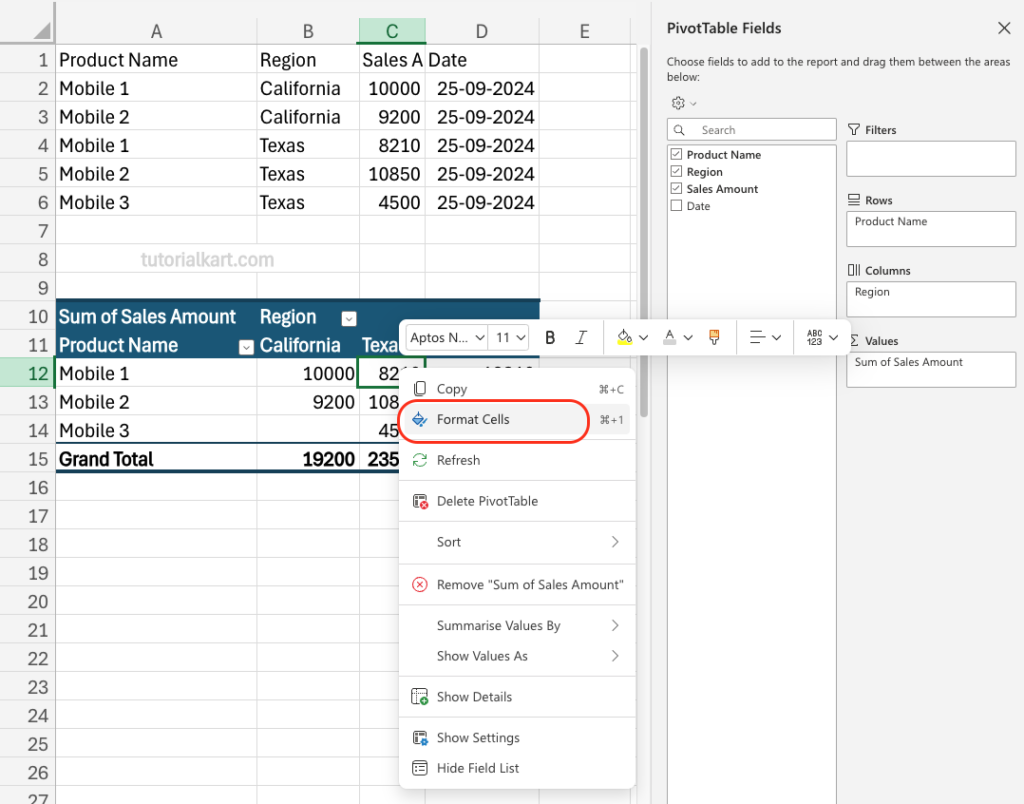
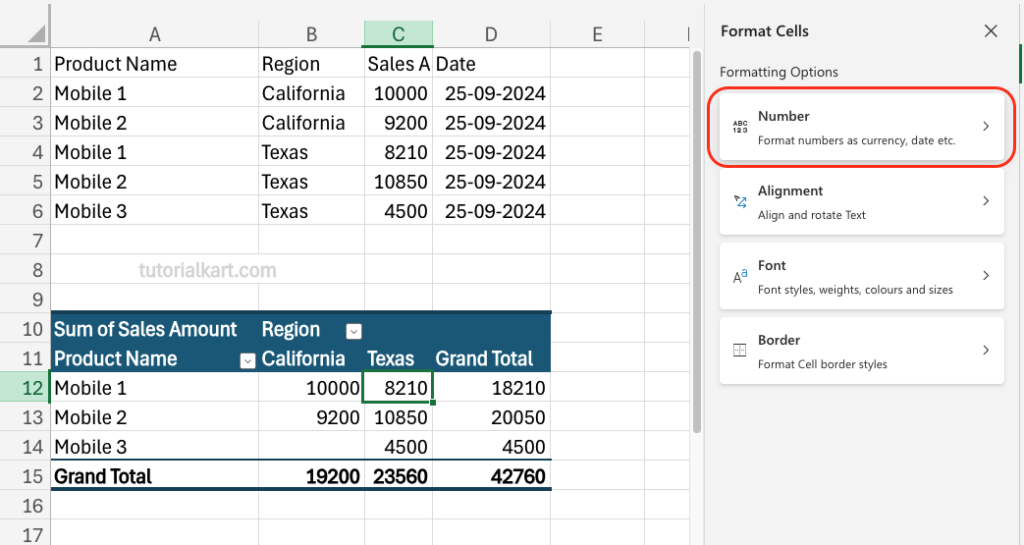
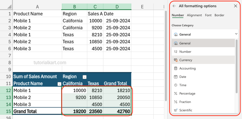
To apply number formatting, right-click on any number in the Values area and select Number Format. You can choose formats such as currency, percentage, or decimal places depending on your data. Let us choose Currency.
To apply conditional formatting, select a range in the pivot table and go to the Home tab. Click on Conditional Formatting to create rules that highlight specific values based on conditions like top/bottom values, data bars, or color scales.
Refreshing Your Pivot Table
One important feature of pivot tables is the ability to refresh the data. If you add new data to the source range or update existing data, you’ll need to refresh the pivot table to see the changes reflected in the report. To refresh your pivot table:
Click anywhere inside the pivot table to bring up the PivotTable Tools tab.
Click on the Analyze tab.
Click Refresh in the Data group.
Excel will update the pivot table based on the changes made to the source data, ensuring that your report remains up-to-date.
Conclusion
Pivot tables are a powerful feature of Excel that can help you quickly analyze and summarize large datasets. Whether you’re calculating sales totals, comparing categories, or filtering data, pivot tables give you the flexibility to manipulate data in various ways.